Confidence intervals for KL divergence (1-D) • kldest

library(kldest)
library(ggplot2)
library(reshape2)
set.seed(0)

We investigate the following pairs of distributions, for which analytical KL divergence values are known:

$\text{Exp}(1)$ vs. $\text{Exp}(1/12)$ ,
$\mathcal{N}(0,1)$ vs. $\mathcal{N}(1,2^2)$ ,
$\mathcal{U}(1,2)$ vs. $\mathcal{U}(0,4)$ .
$\mathcal{U}(0,1)$ vs. $\mathcal{N}(0,1)$ .

p <- list(
    exponential = list(lambda1 = 1, lambda2 = 1/12),
    gaussian    = list(mu1 = 0, sigma1 = 1, mu2 = 1, sigma2 = 2^2),
    uniform     = list(a1 = 1, b1 = 2, a2 = 0, b2 = 4),
    unif_gauss  = list(a = 0, b = 1, mu = 0, sigma2 = 1)
)
distributions <- list(
    exponential = list(
        samples = function(n, m) {
            X <- rexp(n, rate = p$exponential$lambda1)
            Y <- rexp(m, rate = p$exponential$lambda2)
            list(X = X, Y = Y)
        },
        kld = do.call(kld_exponential, p$exponential)
    ),
    gaussian = list(
        samples = function(n, m) {
            X <- rnorm(n, mean = p$gaussian$mu1, sd = sqrt(p$gaussian$sigma1))
            Y <- rnorm(m, mean = p$gaussian$mu2, sd = sqrt(p$gaussian$sigma2))
            list(X = X, Y = Y)
        },
        kld = do.call(kld_gaussian, p$gaussian)
    ),
    uniform = list( 
        samples = function(n, m) {
            X <- runif(n, min = p$uniform$a1, max = p$uniform$b1)
            Y <- runif(m, min = p$uniform$a2, max = p$uniform$b2)
            list(X = X, Y = Y)
        },
        kld = do.call(kld_uniform, p$uniform)
    ),
    unif_gauss = list(
        samples = function(n, m) {
            X <- runif(n, min = p$unif_gauss$a, max = p$unif_gauss$b)
            Y <- rnorm(m, mean = p$unif_gauss$mu, sd = sqrt(p$unif_gauss$sigma2))
            list(X = X, Y = Y)
        },
        kld = do.call(kld_uniform_gaussian, p$unif_gauss)
    )
)

Analytical values for Kullback-Leibler divergences in test cases:

vapply(distributions, function(x) x$kld, 1)
#> exponential    gaussian     uniform  unif_gauss 
#>   1.5682400   0.4431472   1.3862944   1.0856052

Simulation scenarios

For each of the distributions specified above, samples of different sizes are drawn, with several replicates per distribution and sample size.

samplesize <- c(100,1000,10000)
nRep       <- 500L

scenarios <- combinations(
    distribution = names(distributions),
    sample.size  = samplesize,
    replicate    = 1:nRep
)

Algorithm & subsampling methods

The plain 1-NN estimator is considered for this example (according to the 1-D estimation benchmark, there is no expected benefit but additional cost for the bias-reduced version).

estimator <- kld_est_nn

We use the following subsampling methods:

subsmethod <- list(
    sub_n12_q = function(...) kld_ci_subsampling(..., 
                                                 subsample.size = function(n) n^(1/2),
                                                 method = "quantile"), 
    sub_n23_q = function(...) kld_ci_subsampling(..., 
                                                 subsample.size = function(n) n^(2/3),
                                                 method = "quantile"), 
    sub_n12_se = function(...) kld_ci_subsampling(..., 
                                                  subsample.size = function(n) n^(1/2),
                                                  method = "se"),
    sub_n23_se = function(...) kld_ci_subsampling(..., 
                                                  subsample.size = function(n) n^(2/3), 
                                                  method = "se")
)
subsamplingMethodLabels <- c(
    sub_n12_q = "Quantile, s = n^(1/2)",
    sub_n23_q = "Quantile, s = n^(2/3)",
    sub_n12_se = "Std. err., s = n^(1/2)",
    sub_n23_se = "Std. err., s = n^(2/3)"
)
nmethod <- length(subsmethod)

Uncertainty quantification of estimators

Calculation of empirical coverage

# allocating results matrices
nscenario  <- nrow(scenarios)
covered <- matrix(nrow = nscenario, 
                  ncol = nmethod, 
                  dimnames = list(NULL, names(subsmethod)))

# looping over scenarios
for (i in 1:nscenario) {

    dist <- scenarios$distribution[i]
    n    <- scenarios$sample.size[i]
    
    samples <- distributions[[dist]]$sample(n = n, m = n)
    kld     <- distributions[[dist]]$kld
    
    X <- samples$X
    Y <- samples$Y
    
    # all subsampling methods are evaluated on the same samples
    for (j in 1:nmethod) {
        kldboot <- subsmethod[[j]](X, Y, estimator = estimator, B = 500L)
        covered[i,j] <- kldboot$ci[1] <= kld && kld <= kldboot$ci[2]
    }
}

Combine scenarios with CI coverage information:

results <- cbind(scenarios, covered) |> melt(measure.vars  = names(subsmethod),
                                             value.name    = "covered",
                                             variable.name = "subsmethod")

Compute coverage per sample size / subsampling method / distribution:

coverage <- dcast(results, 
                  sample.size + subsmethod + distribution ~ ., 
                  value.var = "covered", 
                  fun.aggregate = function(x) mean(x, na.rm = TRUE))
names(coverage)[4] <- "coverage"

Results: coverage of confidence intervals for KL divergence

ggplot(coverage, aes(x = sample.size, y = coverage, color = subsmethod)) + 
    facet_wrap("distribution") +
    geom_line() + 
    scale_x_log10() +
    geom_hline(yintercept = 0.95, lty = 2) + 
    scale_color_discrete(name = "CI calculation method",
                        labels = subsamplingMethodLabels) +
    ggtitle("Converage of subsampling-based confidence intervals (1-D)") +
    theme(plot.title = element_text(hjust = 0.5))

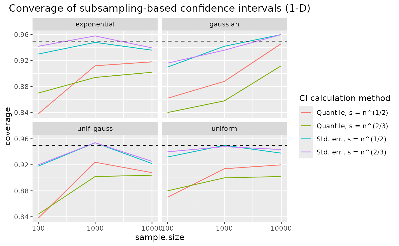
$\Rightarrow$ coverage of the confidence intervals based on nearest neighbour density estimation approaches the nominal coverage of 95% for increasing sample sizes. Coverage is quite robust to the choice of subsample size – which is an argument for using the larger one, $s = n^{(2/3)}$ , since it leads to smaller confidence intervals. Using a subsampling-based estimate of the KL divergence estimator’s standard error in a normal approximation seems to improve coverage compared to the standard quantile method.

Further notes

The above investigated confidence interval calculation method, namely subsampling for a nearest neighbour-based KL divergence estimator, performs best and is recommended. However, other estimators and confidence interval calculation methods are available in the kldest package. Some comments on their performance can be found here.

Confidence intervals for the kernel density-based method

When the kernel density based KL divergence method performs well in the estimation benchmark (such as for Gaussians), confidence intervals also show good coverage properties. However, in cases where the KL divergence estimate shows considerable bias in the estimation benchmark (exponential or uniform distributions), uncertainty quantification also fails. Tailoring the kernel properties (kernel class, bandwidth) to the distribution of interest might allow for improved performance in such cases.

Confidence intervals based on bootstrapping with replacement

Whether to use bootstrapping or subsampling for uncertainty quantification does not play a role for kernel density-based methods – coverage is similar. However, results are dramatically different for nearest neighbour density-based methods, which cannot deal with the ties produced by resampling with replacement.