Comparing 1- vs. 2-sample estimation in 1-D

library(kldest)
library(ggplot2)
library(reshape2)
set.seed(1)

Specification of simulation scenario

Distributions and analytical KL-D

We investigate the following pairs of distributions, for which analytical KL divergence values are known:

• $\text{Exp}(1)$ vs. $\text{Exp}(1/12)$,
• $\mathcal{N}(0,1)$ vs. $\mathcal{N}(1,2^2)$,
• $\mathcal{U}(1,2)$ vs. $\mathcal{U}(0,4)$.

p <- list(
    exponential = list(lambda1 = 1, lambda2 = 1/12),
    gaussian    = list(mu1 = 0, sigma1 = 1, mu2 = 1, sigma2 = 2^2),
    uniform     = list(a1 = 1, b1 = 2, a2 = 0, b2 = 4)
)
distributions <- list(
    exponential = list(
        samples = function(n, m) {
            X <- rexp(n, rate = p$exponential$lambda1)
            Y <- rexp(m, rate = p$exponential$lambda2)
            list(X = X, Y = Y)
        },
        q = function(x) dexp(x, rate = p$exponential$lambda2),
        kld = do.call(kld_exponential, p$exponential)
    ),
    gaussian = list(
        samples = function(n, m) {
            X <- rnorm(n, mean = p$gaussian$mu1, sd = sqrt(p$gaussian$sigma1))
            Y <- rnorm(m, mean = p$gaussian$mu2, sd = sqrt(p$gaussian$sigma2))
            list(X = X, Y = Y)
        },
        q = function(x) dnorm(x, mean = p$gaussian$mu2, sd = sqrt(p$gaussian$sigma2)),
        kld = do.call(kld_gaussian, p$gaussian)
    ),
    uniform = list( 
        samples = function(n, m) {
            X <- runif(n, min = p$uniform$a1, max = p$uniform$b1)
            Y <- runif(m, min = p$uniform$a2, max = p$uniform$b2)
            list(X = X, Y = Y)
        },
        q = function(x) dunif(x, min = p$uniform$a2, max = p$uniform$b2),
        kld = do.call(kld_uniform, p$uniform)
    )
)

Analytical values for Kullback-Leibler divergences in test cases:

vapply(distributions, function(x) x$kld, 1)
#> exponential    gaussian     uniform 
#>   1.5682400   0.4431472   1.3862944

Simulation scenarios

For each of the distributions specified above, samples of different sizes are drawn, with several replicates per distribution and sample size.

samplesize <- 10^(2:4)
nRep       <- 25L

scenarios <- combinations(
    distribution = names(distributions),
    sample.size  = samplesize,
    replicate    = 1:nRep
)

Algorithms

The following algorithms are considered:

algorithms_XY <- list(
    nn_XY     = function(X, Y) kld_est_nn(X, Y)
)
algorithms_Xq <- list(
    nn_Xq = function(X, q) kld_est_nn(X, q = q)
)
nAlgoXY  <- length(algorithms_XY)
nAlgoXq  <- length(algorithms_Xq)
nmAlgo   <- c(names(algorithms_XY),names(algorithms_Xq))

Comparison

Simulation

# allocating results matrices
nscenario  <- nrow(scenarios)
runtime <- kld <- matrix(nrow = nscenario, 
                         ncol = nAlgoXY+nAlgoXq, 
                         dimnames = list(NULL, nmAlgo))

for (i in 1:nscenario) {

    dist <- scenarios$distribution[i]
    n    <- scenarios$sample.size[i]
    
    samples <- distributions[[dist]]$sample(n = n, m = n)
    X <- samples$X
    Y <- samples$Y
    q <- distributions[[dist]]$q

    # different algorithms are evaluated on the same samples
    for (j in 1:nAlgoXY) {
        algo         <- algorithms_XY[[j]]
        start_time   <- Sys.time()
        kld[i,j]     <- algo(X, Y)
        end_time     <- Sys.time()
        runtime[i,j] <- end_time - start_time
    }
    for (j in 1:nAlgoXq) {
        nj            <- nAlgoXY+j
        algo          <- algorithms_Xq[[j]]
        start_time    <- Sys.time()
        kld[i,nj]     <- algo(X, q)
        end_time      <- Sys.time()
        runtime[i,nj] <- end_time - start_time
    }
}

Post-processing: combine scenarios, kld and runtime into a single data frame

tmp1 <- cbind(scenarios, kld) |> melt(measure.vars = nmAlgo,
                                      value.name = "kld",
                                      variable.name = "algorithm") 
tmp2 <- cbind(scenarios, runtime) |> melt(measure.vars = nmAlgo,
                                          value.name = "runtime",
                                          variable.name = "algorithm") 
results <- merge(tmp1,tmp2)
results$sample.size <- as.factor(results$sample.size)
rm(tmp1,tmp2)

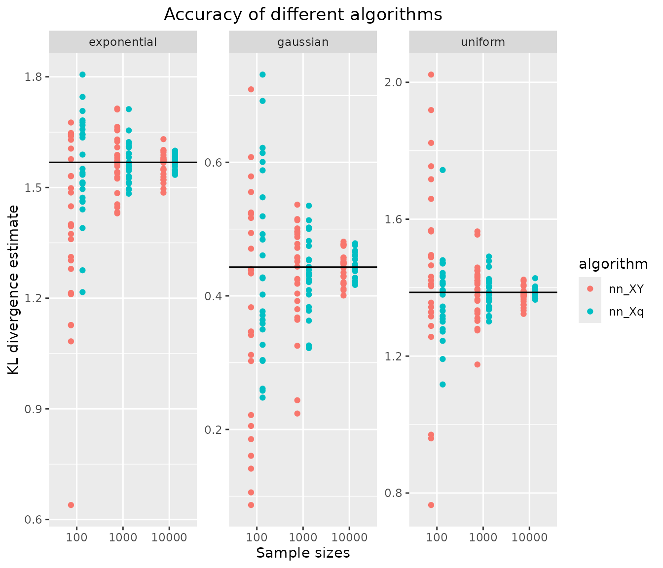
Results: Accuracy of KL divergence estimators

ggplot(results, aes(x=sample.size, y=kld, color=algorithm)) + 
    geom_jitter(position=position_dodge(.5)) + 
    facet_wrap("distribution", scales = "free_y") +
    geom_hline(data = data.frame(distribution = names(distributions), 
                                 kldtrue = vapply(distributions, function(x) x$kld,1)), 
               aes(yintercept = kldtrue)) +
    xlab("Sample sizes") + ylab("KL divergence estimate") + 
    ggtitle("Accuracy of different algorithms") +
    theme(plot.title = element_text(hjust = 0.5))

$\Rightarrow$ 1-sample estimation is more accurate than 2-sample estimation in all three 1-D test cases and for all sample sizes, which is expected since more information is available in the 1-sample case.

However, notice that bias reduction by kld_est_brnn is not possible in 1-sample estimation. Hence, in high-dimensional cases where the density of the approximate distribution $Q$ is available, it may be preferable to simulate a (large) sample from $Q$ and use bias reduction on the two-sample problem, rather than using kld_est_nn in the 1-sample variant.