Algorithm benchmark in high dimensions

library(kldest)
library(ggplot2)
library(reshape2)
library(MASS)
set.seed(0)

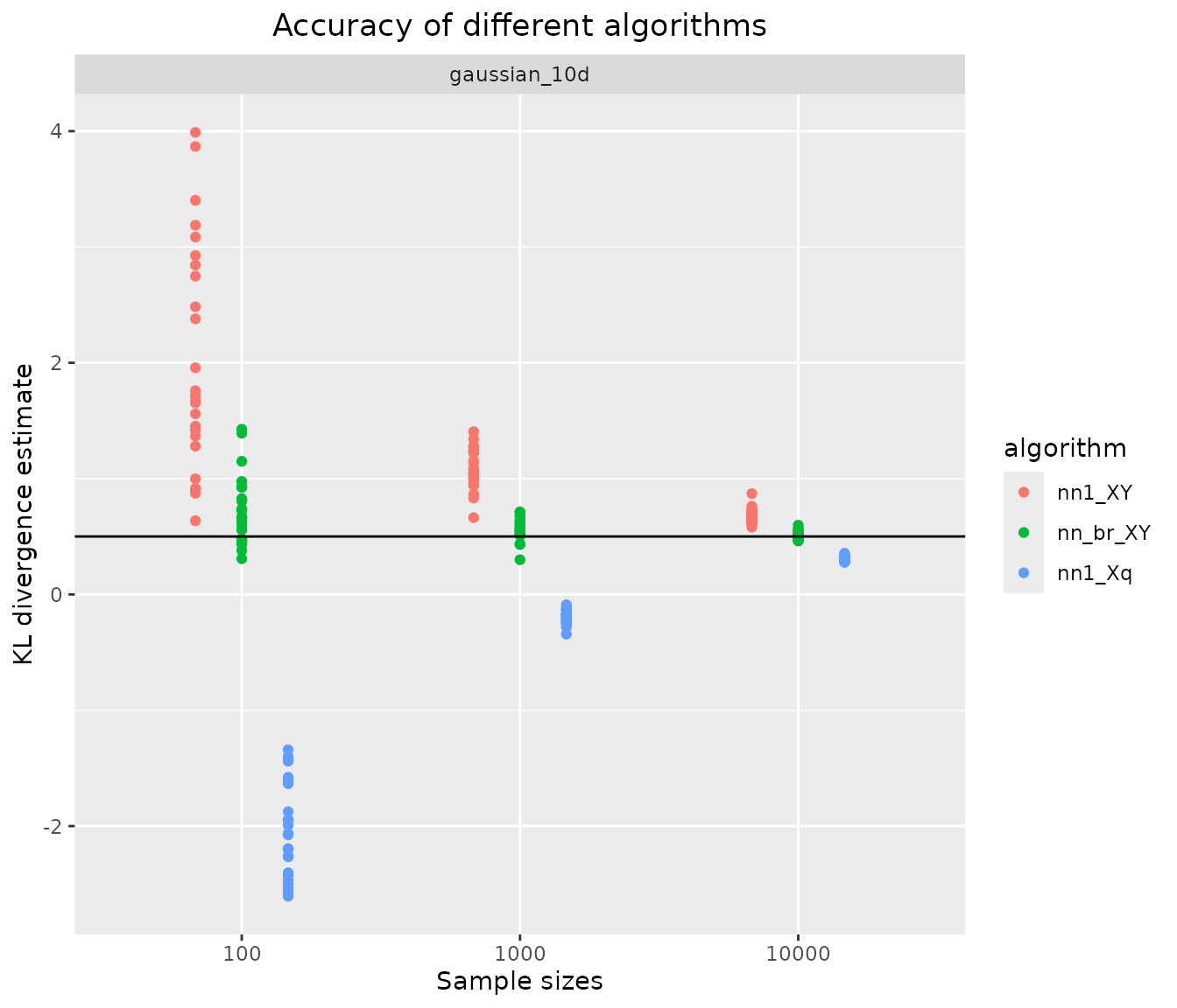
In large dimensions, performance of 1-nearest-neighbour density estimation (one- or two-sample variants) decreases and the bias-reduced variant becomes important. Here, we evaluate a 10-D test case comparing correlated multivariate Gaussians.

Specification of benchmark scenario

Distributions and analytical KL divergence

Simulation study design

D <- 10
Sigma <- constDiagMatrix(dim = D, diag = 1, offDiag = 0.999)

p <- list(
    gaussian_10d = list(
        paramTrue   = list(mu = rep(0, D), sigma = Sigma),
        paramApprox = list(mu = rep(1, D), sigma = Sigma)
    )
)
distributions <- list(
    gaussian_10d = list(
        samples = function(n, m) {
            X <- mvrnorm(n = n, 
                         mu = p$gaussian_10d$paramTrue$mu,   
                         Sigma = p$gaussian_10d$paramTrue$sigma)
            Y <- mvrnorm(n = m, 
                         mu = p$gaussian_10d$paramApprox$mu, 
                         Sigma = p$gaussian_10d$paramApprox$sigma)
            list(X = X, Y = Y)
        },
        q = function(x) mvdnorm(x, mu = p$gaussian_10d$paramApprox$mu, 
                                Sigma = p$gaussian_10d$paramApprox$sigma),
        kld = kld_gaussian(
            mu1    = p$gaussian_10d$paramTrue$mu,
            sigma1 = p$gaussian_10d$paramTrue$sigma,
            mu2    = p$gaussian_10d$paramApprox$mu,
            sigma2 = p$gaussian_10d$paramApprox$sigma)
    )
)

Analytical values for Kullback-Leibler divergences in test cases:

vapply(distributions, function(x) x$kld, 1)
#> gaussian_10d 
#>    0.5004504

Simulation scenarios

For each of the distributions specified above, samples of different sizes are drawn, with several replicates per distribution and sample size.

samplesize <- 10^(2:4)
#n <- c(20,50,100,200,500,1000,2000,5000,10000)
nRep       <- 25L

scenarios <- combinations(
    distribution = names(distributions),
    sample.size  = samplesize,
    replicate    = 1:nRep
)

Algorithms

The following algorithms are considered:

algorithms_XY <- list(
    nn1_XY   = function(X, Y) kld_est_nn(X, Y),
    nn_br_XY = function(X, Y) kld_est_brnn(X, Y, warn.max.k = FALSE)
)
algorithms_Xq <- list(
    nn1_Xq = function(X, q) kld_est_nn(X, q = q)
)
nAlgoXY  <- length(algorithms_XY)
nAlgoXq  <- length(algorithms_Xq)
nmAlgo   <- c(names(algorithms_XY),names(algorithms_Xq))

Run the simulation study

# allocating results matrices
nscenario  <- nrow(scenarios)
runtime <- kld <- matrix(nrow = nscenario, 
                         ncol = nAlgoXY+nAlgoXq, 
                         dimnames = list(NULL, nmAlgo))

for (i in 1:nscenario) {

    dist <- scenarios$distribution[i]
    n    <- scenarios$sample.size[i]
    
    samples <- distributions[[dist]]$sample(n = n, m = n)
    X <- samples$X
    Y <- samples$Y
    q <- distributions[[dist]]$q

    # different algorithms are evaluated on the same samples
    for (j in 1:nAlgoXY) {
        algo         <- algorithms_XY[[j]]
        start_time   <- Sys.time()
        kld[i,j]     <- algo(X, Y)
        end_time     <- Sys.time()
        runtime[i,j] <- end_time - start_time
    }
    for (j in 1:nAlgoXq) {
        nj            <- nAlgoXY+j
        algo          <- algorithms_Xq[[j]]
        start_time    <- Sys.time()
        kld[i,nj]     <- algo(X, q)
        end_time      <- Sys.time()
        runtime[i,nj] <- end_time - start_time
    }
}

Post-processing: combine scenarios, kldiv and runtime into a single data frame

tmp1 <- cbind(scenarios, kld) |> melt(measure.vars  = nmAlgo,
                                      value.name    = "kld",
                                      variable.name = "algorithm") 
tmp2 <- cbind(scenarios, runtime) |> melt(measure.vars  = nmAlgo,
                                          value.name    = "runtime",
                                          variable.name = "algorithm") 
results <- merge(tmp1,tmp2)
results$sample.size <- as.factor(results$sample.size)
rm(tmp1,tmp2)

Graphical display of results

Accuracy of KL divergence estimators

ggplot(results, aes(x=sample.size, y=kld, color=algorithm)) + 
    geom_jitter(position=position_dodge(0.5)) + 
    facet_wrap("distribution", scales = "free_y") +
    geom_hline(data = data.frame(distribution = names(distributions), 
                                 kldtrue = vapply(distributions, function(x) x$kld,1)), 
               aes(yintercept = kldtrue)) +
    xlab("Sample sizes") + ylab("KL divergence estimate") + 
    ggtitle("Accuracy of different algorithms") +
    theme(plot.title = element_text(hjust = 0.5))

$\Rightarrow$ the bias-reduced nearest neighbour algorithm shows much better performance than either of the plain 1-nearest neighbour algorithms. In particular, even if the approximate density q is known (e.g., a model fitted to the data X), it may be preferable to simulate a (large) sample Y from $Q$ and use the bias-reduced algorithm on the two-sample problem, rather than using q.