Algorithm benchmark in 1D • kldest

library(kldest)
library(ggplot2)
library(reshape2)
set.seed(0)

In 1D, different KL divergence estimators are available, either based on kernel density estimation or on nearest-neighbour density estimation. Using different analytically tractable distributions and varying sample sizes, we evaluate different methods in terms of their accuracy and runtime in the two-sample problem.

Specification of benchmark scenario

Distributions and analytical KL divergence

We investigate the following pairs of distributions, for which analytical KL divergence values are known:

$\text{Exp}(1)$ vs. $\text{Exp}(1/12)$ .
$\mathcal{N}(0,1)$ vs. $\mathcal{N}(1,2^2)$ ,
$\mathcal{U}(1,2)$ vs. $\mathcal{U}(0,4)$ ,

p <- list(
    exponential = list(lambda1 = 1, lambda2 = 1/12),
    gaussian    = list(mu1 = 0, sigma1 = 1, mu2 = 1, sigma2 = 2^2),
    uniform     = list(a1 = 1, b1 = 2, a2 = 0, b2 = 4)
)
distributions <- list(
    exponential = list(
        samples = function(n, m) {
            X <- rexp(n, rate = p$exponential$lambda1)
            Y <- rexp(m, rate = p$exponential$lambda2)
            list(X = X, Y = Y)
        },
        kld = do.call(kld_exponential, p$exponential)
    ),
    gaussian = list(
        samples = function(n, m) {
            X <- rnorm(n, mean = p$gaussian$mu1, sd = sqrt(p$gaussian$sigma1))
            Y <- rnorm(m, mean = p$gaussian$mu2, sd = sqrt(p$gaussian$sigma2))
            list(X = X, Y = Y)
        },
        kld = do.call(kld_gaussian, p$gaussian)
    ),
    uniform = list( 
        samples = function(n, m) {
            X <- runif(n, min = p$uniform$a1, max = p$uniform$b1)
            Y <- runif(m, min = p$uniform$a2, max = p$uniform$b2)
            list(X = X, Y = Y)
        },
        kld = do.call(kld_uniform, p$uniform)
    )
)

Analytical values for Kullback-Leibler divergences in test cases:

vapply(distributions, function(x) x$kld, 1)
#> exponential    gaussian     uniform 
#>   1.5682400   0.4431472   1.3862944

Simulation scenarios

For each of the distributions specified above, samples of different sizes are drawn, with several replicates per distribution and sample size.

samplesize <- 10^(2:4)
nRep       <- 25L

scenarios <- combinations(
    distribution = names(distributions),
    sample.size  = samplesize,
    replicate    = 1:nRep
)

Algorithms

We consder the following algorithms:

kernel density estimation with numerical integration (dens_int)
kernel density estimation with a Monte Carlo approximation (dens_mc)
1-nearest neighbour density estimation (nn_1)
bias-reduced nearest neighbour density estimation (nn_br)

algorithms <- list(
    dens_int = function(X, Y) kld_est_kde1(X = X, Y = Y, MC = FALSE),
    dens_mc  = function(X, Y) kld_est_kde1(X = X, Y = Y, MC = TRUE),
    nn_1     = kld_est_nn,
    nn_br = function(X, Y) kld_est_brnn(X = X, Y = Y, warn.max.k = FALSE)
)
nAlgo   <- length(algorithms)

Run the simulation study

# allocating results matrices
nscenario  <- nrow(scenarios)
runtime <- kldiv1d <- matrix(nrow = nscenario, 
                             ncol = nAlgo, 
                             dimnames = list(NULL, names(algorithms)))

for (i in 1:nscenario) {

    dist <- scenarios$distribution[i]
    n    <- scenarios$sample.size[i]
    
    samples <- distributions[[dist]]$sample(n = n, m = n)
    X <- samples$X
    Y <- samples$Y
    
    # different algorithms are evaluated on the same samples
    for (j in 1:nAlgo) {
        algo <- algorithms[[j]]
        start_time <- Sys.time()
        kldiv1d[i,j] <- algo(X, Y)
        end_time <- Sys.time()
        runtime[i,j] <- end_time - start_time
    }
}

Post-processing: combine scenarios, kldiv1d and runtime into a single data frame

tmp1 <- cbind(scenarios, kldiv1d) |> melt(measure.vars = names(algorithms),
                                          value.name = "kld",
                                          variable.name = "algorithm") 
tmp2 <- cbind(scenarios, runtime) |> melt(measure.vars = names(algorithms),
                                          value.name = "runtime",
                                          variable.name = "algorithm") 
results <- merge(tmp1,tmp2)
results$sample.size <- as.factor(results$sample.size)
rm(tmp1,tmp2)

Results

Accuracy of KL divergence estimators

ggplot(results, aes(x=sample.size, y=kld, color=algorithm)) + 
    geom_jitter(position=position_dodge(.5)) + 
    facet_wrap("distribution", scales = "free_y") +
    geom_hline(data = data.frame(distribution = names(distributions), 
                                 kldtrue = vapply(distributions, function(x) x$kld,1)), 
               aes(yintercept = kldtrue)) +
    xlab("Sample sizes") + ylab("KL divergence estimate") + 
    ggtitle("Accuracy of different algorithms") +
    theme(plot.title = element_text(hjust = 0.5))
#> Warning: Removed 10 rows containing missing values or values outside the scale range
#> (`geom_point()`).

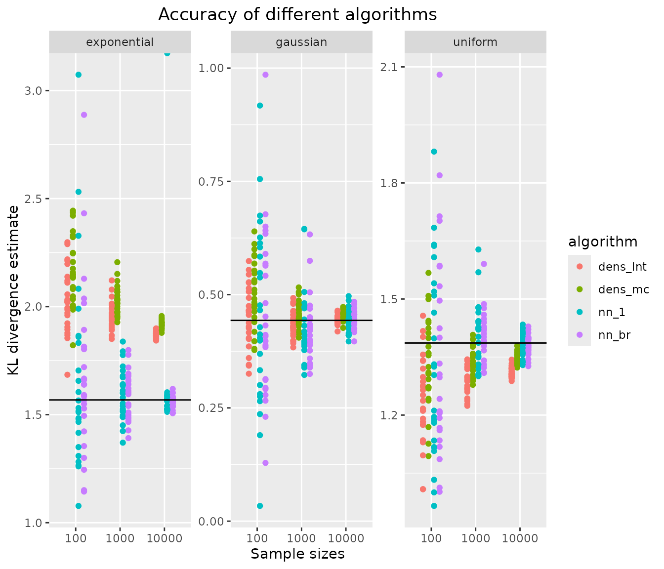
$\Rightarrow$ all estimators converge towards the true KL divergence (black solid line). Kernel density-based estimators generally have a lower variance than nearest neighbour-based estimators, but show some finite sample bias, especially in the asymmetric exponential distribution. There is no difference between the 1-nearest neighbour and bias-reduced k-nearest neighbour methods in terms of accuracy.

Runtime of KL divergence estimators

ggplot(results, aes(x=sample.size, y=runtime, color=algorithm)) + 
    scale_y_log10() + 
    geom_jitter(position=position_dodge(.5)) + 
    facet_wrap("distribution", scales = "free_y") +
    xlab("Sample sizes") + ylab("Runtime [sec]") + 
    ggtitle("Runtime of different algorithms") +
    theme(plot.title = element_text(hjust = 0.5))

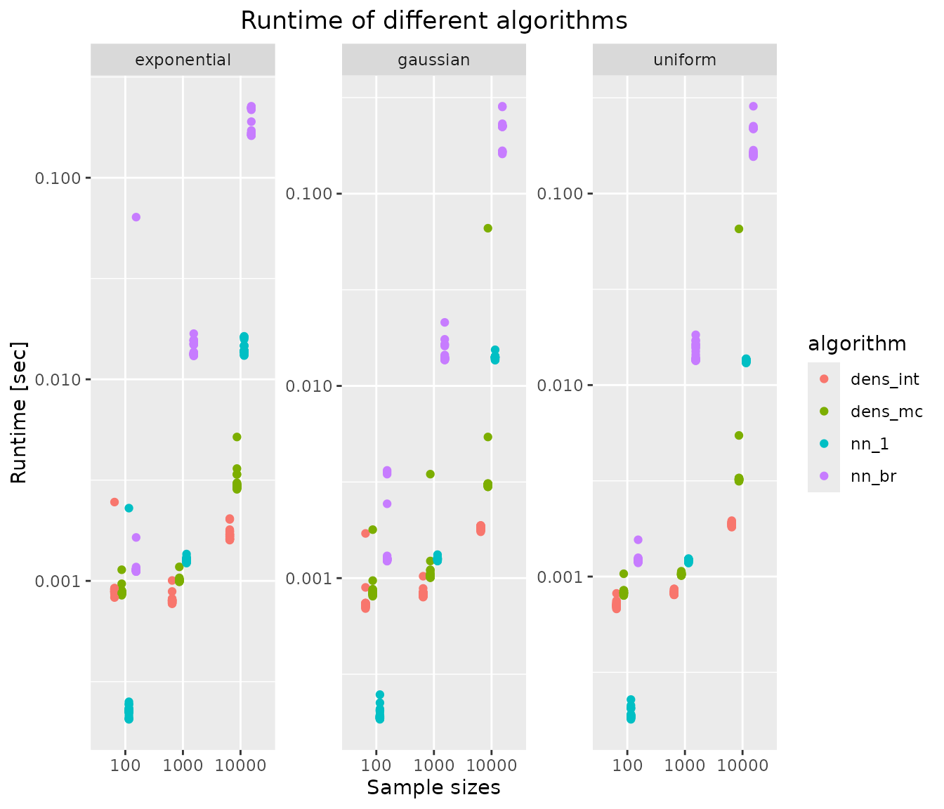
$\Rightarrow$ Kernel density-based estimators, which use stats::density, are generally fastest (except for very small sample sizes). All investigated methods scale approximately linearly with sample size, which is due to the use of a fast Fourier transform in kernel density estimation and use of the kd-tree in the nearest neighbours search. The bias-reduced nearest neighbour estimator nn_br is approximately 1 order of magnitude slower than the 1-nearest neighbour estimator nn_1, without offering additional accuracy in the 1-D examples. The extra effort starts to pay off in higher-dimensional problems.