Confidence intervals for KL divergence (high-dimensional)

Load required packages

library(kldest)
library(ggplot2)
library(MASS)
library(reshape2)

For reproducibility

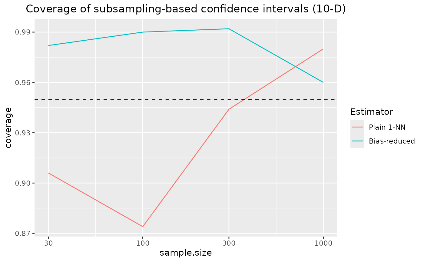
set.seed(0)

We consider two highly correlated Gaussian distributions in 10-D. This is a scenario in which the KL divergence estimation benchmark has shown bias reduction to yield a considerable benefit. Here, we investigate coverage of subsampling based confidence intervals for these two estimators.

D <- 10
Sigma <- constDiagMatrix(dim = D, diag = 1, offDiag = 0.999)

paramTrue   <- list(mu = rep(0, D), sigma = Sigma)
paramApprox <- list(mu = rep(1, D), sigma = Sigma)

sampler <- function(n, param) mvrnorm(n = n, 
                         mu = param$mu,   
                         Sigma = param$sigma)

q <- function(x) mvdnorm(x, 
                         mu = paramApprox$mu, 
                         Sigma = paramApprox$sigma)

Analytical KL-D

kld <- kld_gaussian(
    mu1    = paramTrue$mu,
    sigma1 = paramTrue$sigma,
    mu2    = paramApprox$mu,
    sigma2 = paramApprox$sigma
)

Samples of different sizes are drawn, with several replicates per sample size

samplesize <- c(30,100,300,1000)
nRep       <- 500L
scenarios  <- combinations(
    sample.size  = samplesize,
    replicate    = 1:nRep
)

Subsampling methods

We use the following subsampling methods:

subsmethod <- list(
    sub_nn = function(...) kld_ci_subsampling(..., estimator = kld_est_nn), 
    sub_br = function(...) kld_ci_subsampling(..., estimator = kld_est_brnn)
)
subsamplingMethodLabels <- c(
    sub_nn = "Plain 1-NN",
    sub_br = "Bias-reduced"
)
nmethod <- length(subsmethod)

Uncertainty quantification of estimators

Calculation of empirical coverage

# allocating results matrices
nscenario  <- nrow(scenarios)
covered <- matrix(nrow = nscenario, 
                  ncol = nmethod, 
                  dimnames = list(NULL, names(subsmethod)))

# looping over scenarios
for (i in 1:nscenario) {

    n   <- scenarios$sample.size[i]
    X   <- sampler(n = n, param = paramTrue)
    Y   <- sampler(n = n, param = paramApprox)

    # different algorithms are evaluated on the same samples
    for (j in 1:nmethod) {
        kldboot <- subsmethod[[j]](X, Y, B = 1000L)
        covered[i,j] <- kldboot$ci[1] <= kld && kld <= kldboot$ci[2]
    }
}

Combine scenarios with CI coverage information:

results <- cbind(scenarios, covered) |> melt(measure.vars  = names(subsmethod),
                                             value.name    = "covered",
                                             variable.name = "subsmethod") 

Compute coverage per sample size / algorithm / distribution:

coverage <- dcast(results, 
                  sample.size + subsmethod ~ ., 
                  value.var = "covered", 
                  fun.aggregate = function(x) mean(x, na.rm = TRUE))
names(coverage)[3] <- "coverage"

Results: coverage of confidence intervals for KL divergence

ggplot(coverage, aes(x = sample.size, y = coverage, color = subsmethod)) + 
    geom_line() + 
    scale_x_log10() +
    geom_hline(yintercept = 0.95, lty = 2) + 
    scale_color_discrete(name = "Estimator",
                        labels = subsamplingMethodLabels) +
    ggtitle("Coverage of subsampling-based confidence intervals (10-D)") +
    theme(plot.title = element_text(hjust = 0.5))

$\Rightarrow$ coverage of the confidence intervals based on nearest neighbour density estimation approaches the nominal coverage of 95% for increasing sample sizes.