Algorithm benchmark in 2D • kldest

library(kldest)
library(ggplot2)
library(reshape2)
library(MASS)
set.seed(0)

In this benchmark, the performance of different estimators is evaluated in tractable 2-D examples, in terms of their accuracy and runtime.

The nearest neighbour-based KL divergence estimators shown in the 1-D benchmark are considered again (they are dimension-independent), and a 2-D kernel density-based estimator, relying on package KernSmooth, is
also evaluated.

Specification of simulation scenario

Distributions and KL-D

We investigate the following pairs of distributions, for which analytical KL divergence values are known:

$\mathcal{N}\left(\begin{pmatrix}0\\ 0\end{pmatrix},\begin{pmatrix}1 & 0\\ 0 & 1\end{pmatrix}\right)$ vs. $\mathcal{N}\left(\begin{pmatrix}1\\ 1\end{pmatrix},\begin{pmatrix}2 & 0\\ 0 & 2\end{pmatrix}\right)$ (2D Gaussians, different location/scale, uncorrelated),
$\mathcal{N}\left(\begin{pmatrix}0\\ 0\end{pmatrix},\begin{pmatrix}1 & 0.9\\ 0.9 & 1\end{pmatrix}\right)$ vs. $\mathcal{N}\left(\begin{pmatrix}0\\ 0\end{pmatrix},\begin{pmatrix}1 & 0.1\\ 0.1 & 1\end{pmatrix}\right)$ (2D Gaussians, same location/scale, different correlation strength).

p <- list(
    indep    = list(mu1 = c(0,0), sigma1 = diag(2), 
                    mu2 = c(1,1), sigma2 = 2*diag(2)),
    corr     = list(mu1 = c(0,0), sigma1 = constDiagMatrix(dim = 2, diag = 1, offDiag = 0.9), 
                    mu2 = c(0,0), sigma2 = constDiagMatrix(dim = 2, diag = 1, offDiag = 0.1))
)
distributions <- list(
    indep = list(
        samples = function(n, m) {
            X <- MASS::mvrnorm(n = n, mu = p$indep$mu1, Sigma = p$indep$sigma1)
            Y <- MASS::mvrnorm(n = m, mu = p$indep$mu2, Sigma = p$indep$sigma2)
            list(X = X, Y = Y)
        },
        kld = do.call(kld_gaussian, p$indep)
    ),
    corr = list(
        samples = function(n, m) {
            X <- MASS::mvrnorm(n = n, mu = p$corr$mu1, Sigma = p$corr$sigma1)
            Y <- MASS::mvrnorm(n = m, mu = p$corr$mu2, Sigma = p$corr$sigma2)
            list(X = X, Y = Y)
        },
        kld = do.call(kld_gaussian, p$corr)
    )
)

Analytical values for Kullback-Leibler divergences in test cases:

kldtrue <- data.frame(distribution = factor(names(distributions), 
                                            levels = names(distributions),
                                            ordered = TRUE), 
                      kld          = unname(vapply(distributions, function(x) x$kld,1)))
kldtrue
#>   distribution       kld
#> 1        indep 0.6931472
#> 2         corr 0.7445324

Simulation scenarios

For each of the distributions specified above, samples of different sizes are drawn, with several replicates per distribution and sample size.

samplesize <- 10^(2:5)
nRep       <- 25L

scenarios <- combinations(
    distribution = names(distributions),
    sample.size  = samplesize,
    replicate    = 1:nRep
)

Algorithms

The following algorithms are considered:

algorithms <- list(
    kde2  = function(X, Y) kld_est_kde2(X = X, Y = Y),
    nn_1  = kld_est_nn,
    nn_br = function(X, Y) kld_est_brnn(X = X, Y = Y, warn.max.k = FALSE)
)
nAlgo   <- length(algorithms)

Run the simulation study

# allocating results matrices
nscenario  <- nrow(scenarios)
runtime <- kld <- matrix(nrow = nscenario, 
                         ncol = nAlgo, 
                         dimnames = list(NULL, names(algorithms)))

for (i in 1:nscenario) {

    dist <- scenarios$distribution[i]
    n    <- scenarios$sample.size[i]
    
    samples <- distributions[[dist]]$sample(n = n, m = n)
    X <- samples$X
    Y <- samples$Y
    
    # different algorithms are evaluated on the same samples
    for (j in 1:nAlgo) {
        algo <- algorithms[[j]]
        start_time <- Sys.time()
        kld[i,j] <- algo(X, Y)
        end_time <- Sys.time()
        runtime[i,j] <- end_time - start_time
    }
}

Post-processing: combine scenarios, kld and runtime into a single data frame

tmp1 <- cbind(scenarios, kld) |> melt(measure.vars = names(algorithms),
                                      value.name = "kld",
                                      variable.name = "algorithm") 
tmp2 <- cbind(scenarios, runtime) |> melt(measure.vars = names(algorithms),
                                          value.name = "runtime",
                                          variable.name = "algorithm") 
results <- merge(tmp1,tmp2)
rm(tmp1,tmp2)

Convert to factor

results$sample.size <- as.factor(results$sample.size)
results$algorithm <- factor(results$algorithm, 
                            levels = names(algorithms))
results$distribution <- factor(results$distribution, 
                               levels = names(distributions), 
                               ordered = TRUE)

Results

Accuracy of KL divergence estimators

ggplot(results, aes(x=sample.size, y=kld, color=algorithm)) + 
    geom_jitter(position=position_dodge(.5)) + 
    facet_wrap("distribution", scales = "free_y") +
    geom_hline(data = kldtrue, aes(yintercept = kld)) +
    xlab("Sample sizes") + ylab("KL divergence estimate") + 
    ggtitle("Accuracy of different algorithms") +
    theme(plot.title = element_text(hjust = 0.5))

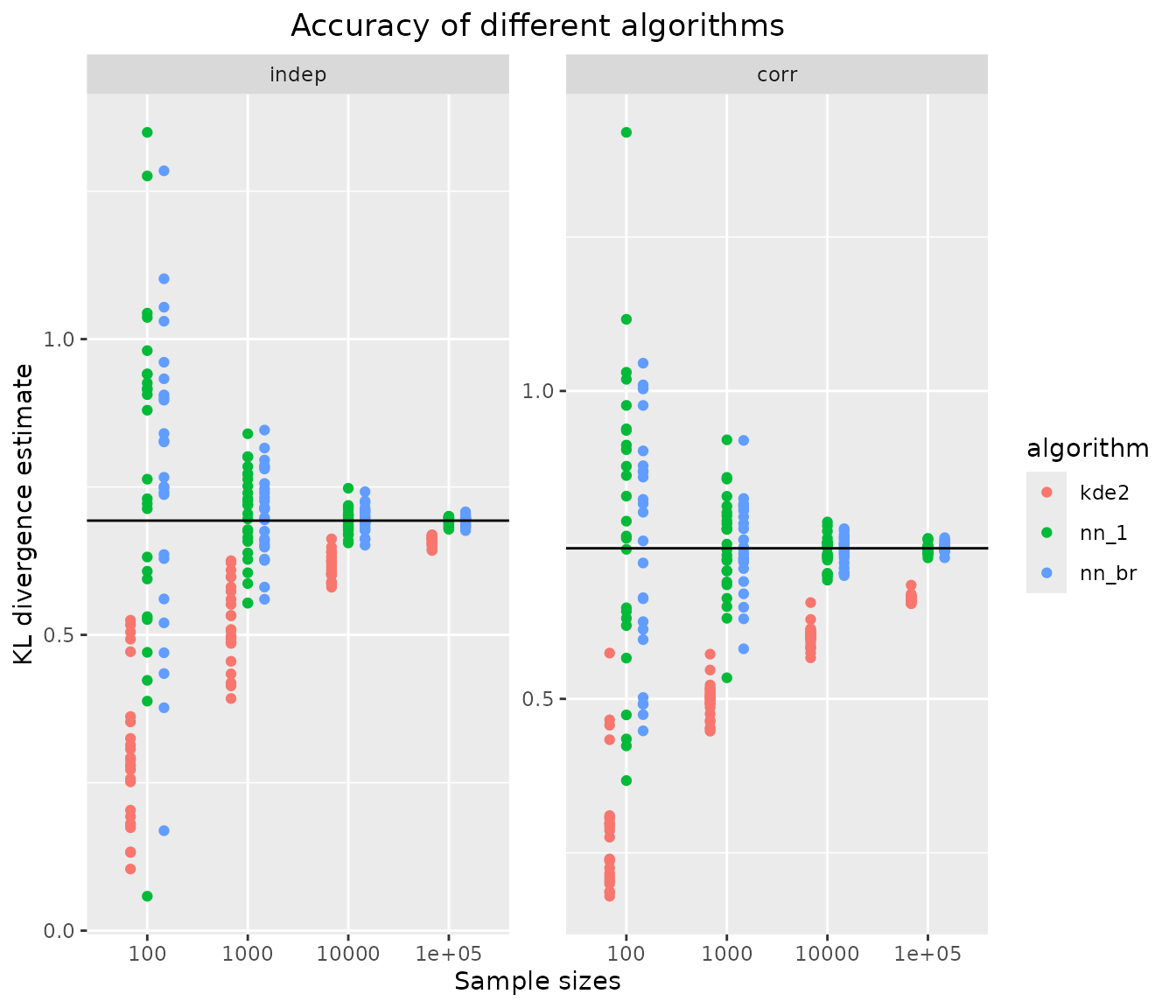
$\Rightarrow$ all estimators converge towards the true KL divergence (black solid line). Whereas both nearest neighbour-based estimators are unbiased, the kernel density-based estimator has comparable variance but considerable bias for smaller samples.

Runtime of KL divergence estimators

ggplot(results, aes(x=sample.size, y=runtime, color=algorithm)) + 
    scale_y_log10() + 
    geom_jitter(position=position_dodge(.5)) + 
    facet_wrap("distribution", scales = "free_y") +
    xlab("Sample sizes") + ylab("Runtime [sec]") + 
    ggtitle("Runtime of different algorithms") +
    theme(plot.title = element_text(hjust = 0.5))

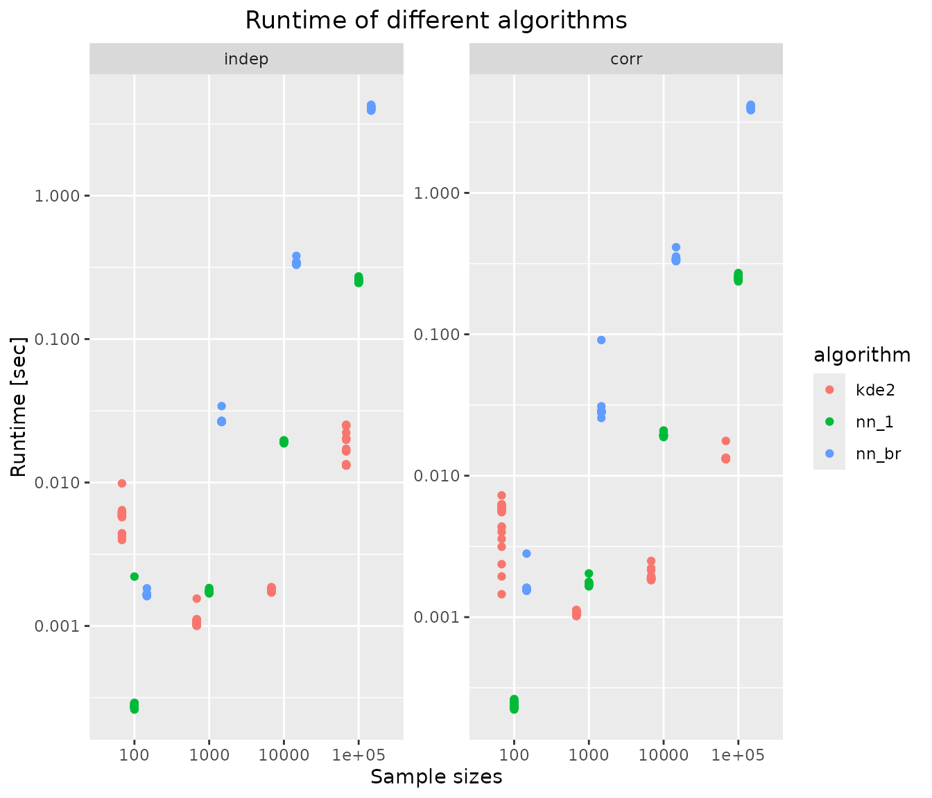
$\Rightarrow$ The kernel density-based estimator, which use KernSmooth::bkde, is more than 10-fold faster than nearest neighbour-based estimators for large samples. However it is also much less precise.